Jonathan Sedar
Personal website and new home of The Sampler blog
Approaches to Data Anonymisation
Editor’s note: this post is from The Sampler archives in 2015. During the last 4 years a lot has changed, not least that now most companies in most sectors have contracted / employed data scientists, and built / bought / run systems and projects. Most professionals will at least have an opinion now on data science, occasionally earned.
Let’s see how well this post has aged - feel free to comment below - and I might write a followup at some point.
Practical data science projects often include an aspect of anonymisation to carefully remove sensitive information prior to analysis; here we demonstrate Bloom filters and complimentary techniques and principles.
Hardly a week goes by without news reports of a security breach at a large organisation and the stealing of sensitive data, recently including Sony Entertainment, Lloyds Bank, and repeated breaches at Talk Talk. The security breaches are often not very sophisticated, and can reveal an amateurish level of security practice within the victim organisations.
In the insurance world, we saw a recent hack into US health insurer Excellus in which attackers gained access to ~10M customer records containing credit card numbers, social security numbers and worryingly, medical histories. Such cyber attacks have been estimated to cost the US health system $6B annually.
Having said that, it’s important that we distinguish such data security from our topic here of data anonymisation:
- Data security generally preserves information content but for a limited audience only; it involves encryption, reduced attack surfaces, operational practices, limits on data-gathering etc
- Data anonymisation generally removes information content, such that the data can be seen safely by a wider audience; it includes removal, obfuscation and aggregation.
Handling sensitive information
Common to both data security and anonymisation is the underlying principle that the information present in data should be available only to the appropriate level of usage by the intended audience.
A large proportion of the information stored about our daily personal and business activities is actually quite sensitive, for example:
| personally identifying | personal attributes | commercially sensitive |
|---|---|---|
| name | gender | client & partner companies |
| home & work address | ethnicity | projects & products |
| telephone number | age | sales & commercial rates |
| email address | marital status | customer details |
| social media handles | education & profession | employee details |
Clearly such information can be used to learn a lot about the behaviour of people and companies, and there are legal and ethical aspects to carefully consider before using any of it, in any form.
Anonymising Structured Data
Assuming that the original data is contained within a well-managed database, the process of extracting data for analysis and anonymising particular fields is technically quite straightforward, but inevitably affects the downstream analysis.
Element-wise feature removal, obfuscation and reduced precision (preserve records)
We seek to remove, obfuscate or reduce the precision of specific fields in such a way that the original information is not part of the copied dataset.
For example, imagine we want to make use of customer information in this (fictional) life policy database:
table: customers

uniqid | first | last  | dob      | gndr | smkr | mrtlstat | postcode
----------------------------------------------------------------------
aa0001 | bob   | smith | 19810123 | M    | N    | single   | EC1V 3EE
af0002 | mark  | jones | 19460802 | M    | S    | widowed  | N8 7TA
cx0003 | anne  | clark | 19581105 | F    | N    | married  | SW1W 9SR
...
At a minimum, good practice will remove direct identifiers - the names in
first and last, and the table key uniqid. We should replace uniqid in
a deterministic way on this primary key and also wherever else it appears as
a foreign key such that we can continue to join tables. A simple, reasonably
fast, infrequently clashing hash function works well e.g. SHA256
It’s also good practice to reduce the precision of the postcode and dob
(date of birth) fields to the minimum useful for analysis; perhaps removing
the latter part of the postcode, and the day and month from the dob. This
helps to prevent directed searches, and may be a simple way of making analyses
more generalisable.
The extracted, record-level anonymised data could look like:
table: extract_customers

newuniqid | yob  | gndr | smkr | mrtlstat | postcode
------------------------------------------------------
zah1034c  | 1981 | M    | N    | single   | EC1V
jgo3332d  | 1946 | M    | S    | widowed  | N8
nnw9298x  | 1958 | F    | N    | married  | SW1W
...
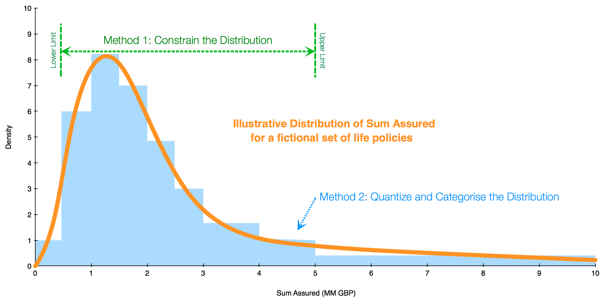
For continuous features like age, salary, sum insured, premium etc, individuals will lie somewhere on a distribution of values and if they happen to be outliers then this too can be a method of identification. For example a life policy may have a sum insured of 10MM GBP, which is likely towards the upper tail of the distribution. We could ‘hide’ this, and other such outliers by:
- constraining the distribution to a maximum such that any values larger than, say, 5MM GBP are limited down to 5MM GBP. The downside is we lose the true distribution which may be important for modelling.
- quantising the distribution into discrete steps, thus the 10MM GBP value may get placed into a categorical band between say, 5MM to 10MM. This again loses fidelity.
Column-wise record aggregation (preserve attributes)
Some information is sufficiently sensitive to warrant aggregating several records together in order to prevent so-called ‘triangulation’, whereby it’s possible to identify an individual based on seemingly-unrelated attributes.1
Taking the example above, the record for Mark Jones might still be identified if we know that he is a widower, born in 1946 and smokes. This combination of attributes may also be rare within the dataset, making a search for his record easier to narrow down.
We undertook a project using the Irish Census. The Census naturally collects some very sensitive socioeconomic data per household including ethnicity, education, employment, health etc. When the Irish Central Statistics Office (CSO) release data back to the public it is strictly in aggregated form only, providing counts summed over several hundred households and preventing triangulation.
Carefully consider the analyses you wish to perform, the questions you seek to answer, and consider whether record aggregation is feasible. In our Census study, the aggregation actually helped the analysis by reducing the volume of data and smoothing out the variability of values within.
The UK Data Archive also has a [good guide](http://www.data-archive.ac.uk/ create-manage/consent-ethics/anonymisation) on structured data anonymisation.
Anonymising Unstructured Data (Pattern Matching)
Freetext is everywhere and with today’s sophisticated text mining & modelling algorithms it’s very tempting to try to use text analysis to gain competitive advantages in everything from public brand engagement, to customer profiling, to recruitment, to improving corporate communications and much more.
However, by it’s nature, unstructured freetext can potentially contain any manner of sensitive information which we often want to remain secure and excluded from analysis.
Regular Expressions
Words are just patterns of characters and therefore just patterns of bytes, and computers are great at matching bytes. The established tool for such text-based pattern matching is regular expressions (regex).
The regex approach works very well when we seek to anonymise an item that obeys a conventional or rules-based structure e.g:
- email address
- phone number
- postcode
- customer ID
- medical ID
For example, if we wanted to remove all email addresses from a lowercased ascii document, we would need to:
- create a generic pattern for an email address, and
- test each word in the document against that pattern, and filter if there is a match
The full email address specification is complicated and to build a real email regex is quite tricky, but lets try to build a very basic pattern here to illustrate.
Assume the basic email address pattern is localname@domainname.tld where:
- there’s always a single
@sign in the middle - the
localnamecan be alphanumerics plus a few symbols - the
domainnamemust start & end with an alphanumeric, may contain hyphens, and it must be less than 63 characters long - the
tld(Top Level Domain) is separated by a fullstop and similarly must start & end with alphanumerics, may contain hyphens and must be fewer than 63 characters long.
The regex mini-language has a reputation for being difficult to write, but if you follow some of the many available guides you can’t go too far wrong. There’s even a handful of online tools like RegExr and regex101 which are handy for one-off testing outside of your codebase.
Accordingly, this very basic (and undoubtedly insufficient) email address regex would contain the patterns:
localname:[a-z0-9!#$%&'*+-/=?^_{}|~]+@:@domainname:[a-z0-9]([a-z0-9-]{0,61}[a-z0-9])?tld:(\.[a-z0-9]([a-z0-9-]{0,61}[a-z0-9])?)?
Python has a great implementation of regex, similar to that of Perl, and so our basic email replacer code could look like:
import re

txt = ('this is a fragment of an email sent from alice@mydomain.com' +
      'to bob@yourdomain.org, which we want to anonymise')

# spec the regex patterns for each part
localname = "[a-z0-9!#$%&'*+-/=?^_{}|~]+"
domainname = "[a-z0-9]([a-z0-9-]{0,61}[a-z0-9])?"
tld = "(\.[a-z0-9]([a-z0-9-]{0,61}[a-z0-9])?)?"

# compile the regex pattern
rx_email = re.compile(localname + '@' + domainname + tld)

# apply the regex to the text, replacing matches with '---'
rx_email.sub('---', txt)

> 'this is a fragment of an email sent from --- to ---, which we want to anonymise'
Next, lets consider how to efficiently anonymise text that doesn’t necessarily obey a fixed pattern.
Anonymising Unstructured Data (Specific Filtering)
This is something more akin to a brute force approach: we create a ‘blacklist’ of words to be removed, and test each word in the document, and removing if it appears in the blacklist.
Such words to exclude via a blacklist might be:
- names of persons
- names of places and addresses
- names of companies and projects
- names of websites
This approach relies on well-maintained blacklists, and they can grow quite large. Alternatively, we could create a ‘whitelist’ of permissible-only words, excluding all words from the document which don’t appear in the list. For example, our whitelist could be comprised of the N most common non-name words in the English language and could be much smaller.
Hash Tables
As the lists of words grows bigger, the computation required for searching
becomes unworkably slow: in an unsorted list the search time scales linearly
with size O(n). Even if we pre-sort the list, which itself takes some time,
O(n log n), a
binary search on a
sorted list can be expected to take O(log n) time.2
A standard solution is to create a
hash table, the most basic version
of which is where the filterlist words are
hashed (mapped to a constant
size) and stored in memory at a location according to the hash value. Now when
we test for membership of the set, all we need to do is hash the query word
and look up the resulting memory location in the set. This takes constant
O(1) time, i.e. the lookup time is independent of the size of the set.
A downside of this approach is that the hash tables can start to get large.
They store all the original information, plus an overhead to avoid hash
collisions. We can demonstrate this easily in Python, using the words
dataset that’s present in most Unix systems:
# NOTE: using Python 3.4 on Mac OSX 10.10.5
# NOTE: using pympler https://github.com/pympler/pympler

from pympler import asizeof

# import Unix `words` list of common English-language words
with open('/usr/share/dict/words','r') as f:
    wrds = ['{}'.format(x.strip().lower()) for x in f.readlines()]

# how many words in the list?
print(len(wrds))
> 235886

# quick look at some of the words in list
print(wrds[50::10000])
> ['abandoner', 'antidiastase', 'beerocracy', 'capriciously'
  , 'commissively', 'deformability', 'el', 'fingal'
  , 'grimalkin', 'hypomanic', 'jillflirt', 'magnesic'
  , 'mousetrap', 'offense', 'passeriform', 'polychromate'
  , 'punctuate', 'ringite', 'shellflower', 'stola'
  , 'tent', 'tyrannoid', 'unoratorial', 'waggishly']

# how much memory does the list consume in bytes?
asizeof.asizeof(wrds)
> 16797448
Our list of words consumes 16.8 MB. Not huge, but already quite unusable for putting into a webpage.
What about a hash table?
# how much memory does the set (hash table) consume in bytes?
asizeof.asizeof(set(wrds))
> 22982240
As expected, the set (hash table) consumes more memory due to overhead: 6.2MB = 37% more. For a whitelist, this large memory footprint might not become too much of a problem, but for a blacklist it might grow beyond a reasonable size.
Perhaps a hash table isn’t enough?
Lets change tack for a minute and imagine that we run a URL shortening service like Bitly or TinyURL. Feed these services with a target URL and they issue a new, shortened URL, e.g. this link https://bit.ly/37a8EUt which makes a web request to Bitly which then redirects to https://insurancedatascience.org. The benefit to the user is an easier to type URL, and the benefit to the Bitly is they get to directly observe the traffic to that 3rd party website and presumably sell that information to advertisers.
Bitly links are apparently 7 case-sensitive alphanumeric characters, creating
a potential search space at (10 numeric + (26 alpha * 2 cases))^7 = 3.5e12
items. Wikipedia notes that as of
August 2018 Bitly has shortened ~3.75 billion (3.75e9) links, so they have
$1-\frac{3.75e9}{3.5e12} \approx 99.89%$ of the search space remaining.
Unending real-estate!
If a user types a short URL which is technically valid but has actually never been issued (e.g. https://bit.ly/37a8EU1), this could cause a wasteful lookup in the Bitly database. Much better to run the requested short URL though a filter or a hash table on the webserver beforehand to test if it has been issued, and only then make the expensive call to the database to return the full normal length URL.
Then again, a hash table with 3.5 trillion entries has a monstrous memory footprint: ascii is 1 byte per char, so 1 * 7 * 3.5e12 = 24 TB
before overhead. Completely infeasible to load into live memory on a webserver.
Now this URL-shortening example is totally contrived, and I’ve no idea if that’s actually how Bitly works, but the principle is in use by several companies and products to speed up database and cache lookups. The trick is to use a Bloom filter, rather than a conventional hash table…
Bloom Filters
A Bloom filter is a space-efficient probabilistic data structure, similar in principle to a hash table but far more compact. We supply the filter with strings and test new strings against it. If a test string has already been added to the filter, then we are guaranteed to get a match (no false negatives). If a test string has never been seen before, then we might get a match (a false positive) with a tuneable probability, $\epsilon$.
We can tune the Bloom filter using the formula:
$$\epsilon \approx (1 - e ^{\frac{-kn}{m}})^k$$
…where:
- $n$ is the number of items to be stored in the filter
- $m$ is the length of the bitarray
- $k$ is the number of hashes each item is put through
As $n$ increases, so does the probability of a false positive, since the filter becomes full and more items test positive. As $m$ increases, there is more room in the filter to store hashes, so $\epsilon$ reduces. There is a conventional setting for $k = \frac{m}{n} ln(2)$
Numerically, we can estimate the storage space required per key as:
$$1.44 log_{2}(\frac{1}{\epsilon})$$
Thus we could create a Bloom filter for our URL-shortening example above, tuned with a false positive rate $\epsilon$ of 1%. This would theoretically require
$$1.44 log_{2}(\frac{1}{0.01}) \approx 9.6 bits \approx 1.2 bytes$$
per item, a total of 1.2 * 3.5e12 = 4.2 TB of memory. This is still pretty
ridiculous in practice, but only 17% of the estimated space required for an
equivalent hash table. Possibly this presents a simpler engineering challenge.
How do Bloom filters work?
In general, a Bloom filter:
- accepts a bytestring to be stored, hashes it a particular number of times in particular ways, and records the resulting hash to an empty bitarray (full of zeros) of fixed size
- the following next item is also put through the same hashing and the final hash is elementwise added to the same bitarray
- if the hash partially collides with the existing bitarray, this is okay and the bitarray simply starts to become full of ones.
For example, lets imagine we’re really bad at shopping and need to use a Bloom filter to determine if we should buy an item. Our shopping list is for apples, bananas and carrots:
import numpy as np

def really_bad_demo_hasher(s):
    """
    Terrible implementation of a hash function to produce
    a bitarray from utf-8 string. For explanation purposes only.
    """

    s_ords = sum([ord(t) for t in s]) # convert string to integer
    s_mod = s_ords % 10               # take mod 10
    s_arr = np.zeros(10)              # create empty bitarray
    s_arr[s_mod] = 1                  # set bitarray according to string

    return s_arr


# fill Bloom filter with a short shopping list of fruit & veg

bf = np.zeros(10)

for item in ['apples','bananas','carrots']:
    item_bitarr = really_bad_demo_hasher(item)
    print('{} {}'.format(item_bitarr,item))
    bf += item_bitarr

print('\n{} {}'.format(bf,'total'))


> [ 0.  0.  0.  0.  0.  1.  0.  0.  0.  0.] apples
  [ 0.  0.  0.  0.  1.  0.  0.  0.  0.  0.] bananas
  [ 0.  0.  0.  0.  0.  0.  1.  0.  0.  0.] carrots

  [ 0.  0.  0.  0.  1.  1.  1.  0.  0.  0.] total
Here you can see each item in the list of fruits and vegetables gets hashed
once $k=1$ and added to the Bloom filter bf, which starts to fill with ones.
Now we have the shopping list we’ll walk around the supermarket, testing the items we find. If the Bloom filter responds with a match, then we should buy the item:
def test_bloomfilter(bf, s):
    """
    Test if string `s` is in Bloomfilter `bf`
    """
    if min( bf - really_bad_demo_hasher(s)) < 0:
        return 'Nope, no {} today'.format(s)
    else:
        return 'Yes, {} are on the list, buy them!'.format(s)


for item in ['oranges', 'bananas', 'eggplants']:
    print(test_bloomfilter(bf, item))

> Nope, no oranges today
  Yes, bananas are on the list, buy them!
  Yes, eggplants are on the list, buy them!
Great, we didn’t want oranges and we did want bananas, good so far. However we seem to be about to buy eggplants, which definitely wasn’t on the list!
This false positive is a direct result of the way that Bloom filters work, in this case the hash for ‘eggplants’ looks the same as that for ‘apples’, which is on the list:
for item in ['apples', 'eggplants']:
    item_bitarr = really_bad_demo_hasher(item)
    print('{} {}'.format(item_bitarr,item))

> [ 0.  0.  0.  0.  0.  1.  0.  0.  0.  0.] apples
  [ 0.  0.  0.  0.  0.  1.  0.  0.  0.  0.] eggplants
The simple solution to this is to increase the size of the bitarray $m$.
A more realistic example
Lets say we have a large document and are concerned that it might contain the names of people who should otherwise be anonymous. We want to remove these names.
I’ll use a big list of first and last names which I partially created using freely available lists of names from the 1990 USA Census. Ask if you’d like access.
My list contains 6046 first names, and 156360 last names, totalling 162,406 strings. What memory footprint can we expect to need for a conventional Bloom filter if we require a low false positive rate $\epsilon = 0.1%$?
$$1.44 * log_{2}(\frac{1}{0.001}) \approx 14.35\text{bits} \approx 1.79 \text{bytes}$$
$$1.79 * 162406 \text{string} \approx 291kB$$
Lets check what we get when using the pybloom package:
from pybloom import BloomFilter

bf = BloomFilter(capacity=len(names), error_rate=0.001)

print('Filter consumes approx {:,.0f} bytes'.format(bf.num_bits/8))

> Filter consumes approx 291,876 bytes

# how big is the hash table (bytes)?
asizeof.asizeof(set(names))

> 13673544
The Python pybloom implementation appears to be very close to the
theoretical size of the Bloom filter, and is a fraction of the size of the
hash table: $\frac{292kB}{13674kB} \approx 2.14%$
To complete the comparison, let’s take a look at the runtime required to parse through some real text:
import requests

# get real-world text document "The Adventures of Sherlock Holmes"
sherlock = requests.get('https://www.gutenberg.org/cache/epub/1661/pg1661.txt').text

# initialise Bloom filter
bf = BloomFilter(capacity=len(names), error_rate=0.001)
print('Filter setup with {:.1e} bits, capacity for {} items'.format(
        bf.num_bits, bf.capacity))

> Filter setup with 2.3e+06 bits, capacity for 162406 items

# populate bloomfilter and hash table
_ = [bf.add(w) for w in names]
setnames = set(names)

# time duration for applying hash table to Sherlock text
%timeit ['REM' if t.lower() in setnames else t for t in sherlock.split()]

> 10 loops, best of 3: 34.8 ms per loop

# time duration for applying bloomfilter on Sherlock text
%timeit ['REM' if t.lower() in bf else t for t in sherlock.split()]

> 1 loops, best of 3: 380 ms per loop
Here we see the Bloom filter takes 380ms to filter the text - approx 11x
slower than the hash table - likely due to the number of hash operations $k$
required to test each item in the Bloom filter.
Clearly there’s a trade-off to make between memory footprint and execution time.
Summary
There’s a lot of detail in data anonymisation.
-
If the data is structured then we can apply certain techniques to either preserve records or preserve features, while making it hard to identify individuals
-
If the data is unstructured, we can apply pattern matching and filtering to remove sensitive information.
All throughout, there’s tradeoffs to make which affect the downstream analysis and the audience that may see such analyses. Key to all is the principle that we only ever store, access and use the appropriate level of information for the task at hand.
-
The Electronic Freedom Foundation discovered in 2010 that approx. 8 in 10 internet browsers are uniquely identifiable amongst all other browsers in the world. Each browser has a ‘fingerprint’ based on a combination of details given to a webserver when it requests a page. Though no single attribute is especially informative - e.g. operating system, language, fonts, screen size - they create a lot of information when combined. I just tested my browser using the EFF’s online service Panopticlick and it has a fingerprint that is apparently unique amongst the ~245k browsers tested in the last 45 days, and carries ~18 bits of identifying information, sufficient to distinguish it within a pool of up to $2^{18} = 260k$ browsers. ↩︎
-
Such ‘Big-O’ notation is a standard way to indicate the running time of an algorithm, with respect to the number of items processed, n. ↩︎